Sorting
sorting은 array에 저장되어 있는 원소들을 값이 커지는 순서 혹은 값이 작아지는 순서로 재배열하는 것을 의미한다.
sorting에는 각각의 원소를 비교하여 해당 원소보다 큰지 작은 지를 확인해야 하기 때문에 relational operator가 잘 정의돼야 한다.
아래의 정렬 방법들을 살펴볼 때 오름차순과 내림차순은 단순히 정렬하는 순서를 바꾸면 동일함으로 모든 경우 오름차순으로 정렬함을 가정하겠다.
- Selection Sort
가장 기본적인 정렬 방법으로 정렬되지 않은 array에서 가장 작은 값을 찾은 뒤 해당하는 값을 정렬되어 있는 배열의 뒤로 붙이는 방법이다.
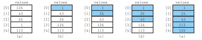
만약 N개의 배열을 selection sort를 사용하여 정렬한다면 $\sum\limits_{i = 1}^{N - 1} i = \frac{N(N - 1)}{2}$ 이므로 시간복잡도가 $O(N^2)$이 나온다.
구현하는 방법은 정렬되지 않은 배열에서 가장 작은 원소가 속한 인덱스를 찾아내고 해당 인덱스의 값을 정렬되지 않은 배열의 가장 앞의 인덱스의 값과 swap 해준다.
이때 가장 마지막 원소는 앞의 N - 1개의 원소가 정렬되어 있으면 자동으로 정렬됨으로 마지막 원소 전까지만 정렬해 주면 된다.
int MinIndex(ItemType values[], int startIndex, int endIndex) {
	int indexOfMin = startIndex;
	for (int index = startIndex + 1; index <= endIndex; index++)	{
		if (strcmp(values[index].getName(),values[indexOfMin].getName()) < 0)
			indexOfMin = index;
	}
	return indexOfMin;
}

void SelectionSort(ItemType ary[], int numElems) {
	int endIndex = numElems - 1;
	for (int current = 0; current < endIndex; current++)
		Swap(ary[current], ary[MinIndex(ary, current, endIndex)]);
}
파이썬으로도 코딩하면 다음과 같다.
def selection_sort(values):
    for i in range(len(values) - 1):
        indexofmin = i
        for j in range(i + 1, len(values)):
            if values[j] < values[indexofmin]:
                indexofmin = j
            values[i], values[indexofmin] = values[indexofmin], values[i]
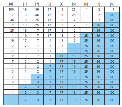
- Bubble Sort
bubble sort는 배열의 가장 아래에 있는 원소와 그 원소의 바로 앞의 원소를 비교하여 만약 뒤에 있는 원소가 더 작을 경우 두 원소의 값을 swap 해주고 이제 그 앞에 있는 원소와 이러한 과정을 정렬된 배열에 도달할 때까지 반복하여 원소를 정렬하는 방법이다.
이러한 방법 때문에 비교할수록 거품처럼 뒤에 있던 원소들이 올라온다는 이유로 bubble sort라고 한다.
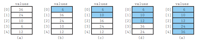
bubble sort는 selection sort와 동일한 횟수의 연산이 필요함으로 시간 복잡도는 $O(N^2)$이 나온다.
void BubbleUp(ItemType values[], int startIndex, int endIndex) {
	for (int index = endIndex; index > startIndex; index--) {
		if (strcmp(values[index].getName(), values[index - 1].getName()) < 0)
			Swap(values[index], values[index - 1]);
	}
}

void BubbleSort(ItemType ary[], int numElems) {
	int current = 0;
	while (current < numElems - 1)	{
		BubbleUp(ary, current, numElems - 1);
		current++;
	}
}
파이썬으로도 코딩하면 다음과 같다.
def bubble_sort(values):
    for i in range(len(values) - 1, 0, -1):
        for j in range(i):
            if values[j] > values[j + 1]:
values[j], values[j + 1] = values[j + 1], values[j]- Insertion Sort
insertion sort는 정렬되지 않은 array의 가장 앞에 있는 원소를 바로 앞에 있는 정렬된 array와 비교하여 정렬된 배열에서 삽입되기 적절한 위치를 찾은 뒤 해당하는 부분에 삽입되는 정렬 방식이다.
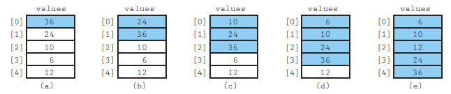
insertion sort의 시간 복잡도는 array가 원래 정렬되어 있었을 경우 $O(N)$으로 최소가 나오지만 이러한 경우는 거의 없으므로 일반적인 경우를 생각하면 selection sort와 동일한 횟수의 연산이 필요하여 $O(N^2)$의 시간 복잡도가 나오게 된다.
insertion sort를 구현할 때 삽입되기 적절한 위치를 찾은 다음 삽입을 하려면 해당 부분에 공간을 만들어 주기 위해 원소들을 뒤로 이동시켜야 하는 과정이 필요하기 때문에 찾는 과정과 삽입하는 과정을 따로 하는 것이 아니라 bubble sort와 유사한 방법으로 원소를 하나씩 비교하여 작은 원소가 앞으로 오게 swap해주는 방식을 사용하면 된다.
void InsertItem(Student values[], int startIndex, int endIndex) {
	bool finished = false;
	int current = endIndex;
	bool moreToSearch = (current != startIndex);
	while (moreToSearch && !finished) {
		if (strcmp(values[current].getName(), values[current - 1].getName()) < 0) {
			Swap(values[current], values[current - 1]);
			current--;
			moreToSearch = (current != startIndex);
		}
		else
			finished = true;
	}
}

void InsertionSort(Student ary[], int numElems) {
	for (int count = 0; count < numElems; count++)
		InsertItem(ary, 0, count);
}
파이썬으로 코딩하면 다음과 같다.
def insertion_sort(values):
    for i in range(1, len(values)):
        for j in range(i, 0, -1):
            if values[j - 1] > values[j]:
                values[j - 1], values[j] = values[j], values[j - 1]
- Heap Sort
heap sort는 array가 주어지면 해당 배열을 heap으로 만들고 root가 가장 큰 원소를 가리키고 있으므로 root의 값과 정렬이 안된 array의 가장 마지막 원소의 값을 바꿔주면 오름차순으로 정렬이 된다.
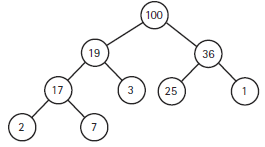
heap에서 root에 있는 원소를 마지막 값과 바꾸면 정렬이 안된 array를 다시 heap구조로 바꾸기 위해서 ReheapDown을 수행한다.
heap sort를 수행하기 위해서는 일단 array를 heap으로 만들어줘야 한다.
기본적으로 tree를 array로 표현할 때 parent node를 i라고 할 때 right child node는 $2 \times i + 1$, left child node는 $2 \times i + 2$가 된다.
따라서 parent node들은 array의 전체의 길이가 N일 때 index가 0부터 $\frac {N}{2} - 1$인 위치에 있게 된다.
따라서 array를 heap으로 만들기 위해서 해당하는 모든 parent node의 가장 아래부터 ReheapDown을 수행하게 되면 자동으로 array가 heap구조를 가지게 된다.
따라서 전체 시간 복잡도는 처음에 heap을 만들기 위해서 ReheapDown이 $O(\log(N))$이 소요되고 이러한 과정을 $\frac {N}{2} - 1$번 반복함으로 총 시간 복잡도는 $O(N \log(N))$이고, heap sort를 수행하면 ReheapDown을 N - 1번 수행하여 $O(N \log(N))$ 따라서 총 $O(N \log(N))$만큼 소요된다.
template<class ItemType>
void ReheapDown(ItemType elements[], int root, int bottom) {
	int maxChild;
	int rightChild;
	int leftChild;
	leftChild = root * 2 + 1;
	rightChild = root * 2 + 2;
	if (leftChild <= bottom) {
		if (leftChild == bottom)
			maxChild = leftChild;
		else {
			if (elements[leftChild] <= elements[rightChild])
				maxChild = rightChild;
			else
				maxChild = leftChild;
		}
		if (elements[root] < elements[maxChild]) {
			Swap(elements[root], elements[maxChild]);
			ReheapDown(elements, maxChild, bottom);
		}
	}
}

template<class ItemType>
void HeapSort(ItemType values[], int numValues) {
	int index;
	for (index = numValues / 2 - 1; index >= 0; index--)
		ReheapDown(values, index, numValues - 1);
	for (index = numValues - 1; index >= 1; index--) {
		Swap(values[0], values[index]);
		ReheapDown(values, 0, index - 1);
	}
}
이를 파이썬으로 구현하면 다음과 같다.
def reheap_down(elements, root, bottom):
    leftchild = root * 2 + 1
    rightchild = root * 2 + 2
    if leftchild <= bottom:
        if leftchild == bottom:
            maxchild = leftchild
        else:
            if elements[leftchild] <= elements[rightchild]:
                maxchild = rightchild
            else:
                maxchild = leftchild
        if elements[root] < elements[maxchild]:
            elements[root] , elements[maxchild] = elements[maxchild], elements[root]
            reheap_down(elements, maxchild, bottom)

def heap_sort(values, numValues):
    for i in range(numValues // 2 - 1, -1, -1):
        reheap_down(values, i, numValues - 1)
    for j in range(numValues - 1, 0, -1):
        values[0], values[j] = values[j], values[0]
        reheap_down(values, 0, j - 1)
- Quick Sort
quick sort는 대표적인 분할 정복 알고리즘이다.
quick sort의 동작 과정은 먼저 제일 앞의 요소를 pivot으로 지정하고 pivot을 제외하고 array에서 가장 앞부분을 가리키는 first와 뒷부분을 가리키는 last를 얻는다.
그리고 first에서부터 array를 쭉 탐색하여 pivot보다 큰 값이 나오는 위치를 찾고, last부터 array를 탐색하여 pivot보다 작은 값이 나오는 위치를 찾는다.
이때 first와 last의 순서가 아직 바뀌지 않았으면 찾은 두 값을 서로 swap 하여 왼쪽 부분에는 pivot보다 작은 값들의 모임이, 오른쪽에는 pivot보다 큰 값들의 모임이 생기게 만들고 다시 fisrt와 last위치에서부터 탐색을 시작하여 pivot보다 크거나 작은 값이 나오는 위치를 찾는 과정을 반복한다.
그러다 만약 first와 last의 순서가 서로 바뀌게 된다면 pivot을 기준으로 array에서 해당 값보다 작은 값은 왼쪽 부분에 모두 다 있고, 해당 값 보다 큰 값은 오른쪽 부분에 모두 다 있다는 것을 의미한다.
따라서 pivot을 해당 부분에 집어넣으면 array에서 pivot이 들어갈 적절한 위치를 얻게 되고, 이제 왼쪽과 오른쪽 array에 대해 각각 다시 quick sort를 진행하면 모든 원소들이 array에서 알맞은 위치로 정렬이 된다.
quick sort의 시간 복잡도를 살펴보면 처음에 $N$개의 노드를 살펴보고, 그 다음은 2개의 $\frac{N}{2}$개의 노드를 살펴보고, 그다음은 4개의 $\frac{N}{4}$의 노드를 살펴보는 과정을 총 $\log_2(N)$번 반복함으로 결과적으로 매번 $N$개의 노드를 $\log_2(N)$번 반복하여 전체 시간 복잡도는 $N \log_2(N)$이 나온다.
다만 이는 이상적인 경우로 split을 하였을 때 매번 절반씩 나눠지는 경우를 나타낸다.
만약 최악의 경우로 이미 정렬된 array에 quick sort를 적용하게 되면 매번 $N$개의 노드를 $N$번 반복하여 전체 시간 복잡도는 $N^2$이 나온다.
void Split(ItemType values[], int first, int last, int& splitPoint) {
	ItemType splitVal = values[first];
	int saveFirst = first;
	bool onCorrectSide;
	first++;
	do {
		onCorrectSide = true;
		while (onCorrectSide) {
			if (strcmp(splitVal.getName(), values[first].getName()) < 0) {
				onCorrectSide = false;
			}
			else {
				first++;
				onCorrectSide = (first <= last);
			}
		}
		onCorrectSide = true;
		while (onCorrectSide) {
			if (strcmp(splitVal.getName(), values[last].getName()) > 0) {
				onCorrectSide = false;
			}
			else {
				last--;
				onCorrectSide = (first <= last);
			}
		}
		if (first < last) {
			Swap(values[first], values[last]);
			first++;
			last--;
		}
	} while (first <= last);
	splitPoint = last;
	Swap(values[saveFirst], values[splitPoint]);
}

void QuickSort(ItemType values[], int first, int last) {
	if (first < last) {
		int splitPoint;
		Split(values, first, last, splitPoint);
		QuickSort(values, first, splitPoint - 1);
		QuickSort(values, splitPoint + 1, last);
	}
}
이를 파이썬으로 다시 구현하면 다음과 같다.
def split(values, first, last):
    splitval = values[(first + last) // 2]
    while first <= last:
        while values[first] < splitval:
            first += 1
        while values[last] > splitval:
            last -= 1
        if first <= last:
            values[first], values[last] = values[last], values[first]
            first, last = first + 1, last - 1
    return first

def quick_sort(values, first, last):
    if first < last:
        mid = split(values, first, last)
        quick_sort(values, first, mid-1)
quick_sort(values, mid, last)- Merge Sort
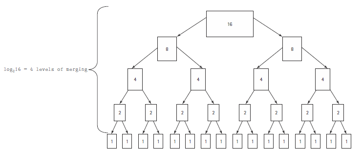
merge sort또한 대표적인 분할 정복 알고리즘이다.
merge sort의 동작 과정은 먼저 array를 절반으로 나누고 왼쪽 부분을 정렬하고 오른쪽 부분을 정렬한 다음에 두 array를 다시 병합하는 아이디어를 사용한다.
절반을 분할하여 나눠진 배열을 정렬하기 위해서 또 merge sort를 사용하여 재귀적으로 분할을 하는데 분할된 배열의 원소의 수가 1개여서 더 이상 분할을 할 수 없을 때까지 계속 분할을 한다.
이제 배열을 병합해줘야 하는데 새로운 배열을 만들어 두 배열의 원소를 작은 값 부터 비교하여 둘 중 작은 값을 새로운 배열에 삽입한다.
삽입된 원소가 있는 배열은 이미 정렬되어 있으므로 해당 원소의 다음 값과 다른 배열의 비교했던 값을 비교하여 또 작은 값을 새로운 배열에 삽입하는 과정을 한쪽 배열의 원소가 없어질 때까지 반복한다.
만약 한 쪽 배열의 원소가 모두 삽입되어 남지 않았다면 반대편 배열은 새로운 배열의 모든 값보다 큰 값이 정렬되어 있으므로 해당 배열을 새로운 배열 뒤에 그대로 병합해 준다.
이제 이러한 과정을 새로운 배열이 전체 배열이 전체 배열의 정렬과 같아질 때까지 계속 반복한다.
merge sort의 시간 복잡도를 보면 quick sort의 이상적인 과정과 똑같은 연산 횟수가 필요함으로 총 $N \log_2(N)$의 시간 복잡도가 나온다.
void Merge(ItemType values[], int leftFirst, int leftLast, int rightFirst, int rightLast) {
	int arySize = rightLast - leftFirst + 1;
	ItemType* tempArray = new ItemType[arySize];
	int index = 0;
	int saveFirst = leftFirst;
	while ((leftFirst <= leftLast) && (rightFirst <= rightLast)) {
		if (strcmp(values[leftFirst].getName(), values[rightFirst].getName()) <= 0) {
			tempArray[index] = values[leftFirst];
			leftFirst++;
		}
		else {
			tempArray[index] = values[rightFirst];
			rightFirst++;
		}
		index++;
	}
	while (leftFirst <= leftLast) {
		tempArray[index] = values[leftFirst];
		leftFirst++;
		index++;
	}
	while (rightFirst <= rightLast) {
		tempArray[index] = values[rightFirst];
		rightFirst++;
		index++;
	}
	for (index = saveFirst; index <= rightLast; index++)
		values[index] = tempArray[index - saveFirst];

	delete[] tempArray;
	_CrtDumpMemoryLeaks();
}

void MergeSort(ItemType values[], int first, int last) {
	if (first < last) {
		int middle = (first + last) / 2;
		MergeSort(values, first, middle);
		MergeSort(values, middle + 1, last);
		Merge(values, first, middle, middle + 1, last);
	}
}
이를 파이썬으로 코딩하면 다음과 같다.
def merge(values, leftFirst, leftLast, rightFirst, rightLast):
    tempArray = []
    savefirst = leftFirst
    while(leftFirst <= leftLast and rightFirst <= rightLast):
       if (values[leftFirst] < values[rightFirst]):
           tempArray.append(values[leftFirst])
           leftFirst += 1
       else:
           tempArray.append(values[rightFirst])
           rightFirst += 1
    while (leftFirst <= leftLast):
        tempArray.append(values[leftFirst])
        leftFirst += 1
    while (rightFirst <= rightLast):
        tempArray.append(values[rightFirst])
        rightFirst += 1
    for i in range(savefirst, rightLast + 1):
        values[i] = tempArray[i - savefirst]

def merge_sort(values, first, last):
    if first < last:
        middle = (first + last) // 2
        merge_sort(values, first, middle)
        merge_sort(values, middle + 1, last)
merge(values, first, middle, middle + 1, last)- Radix Sort
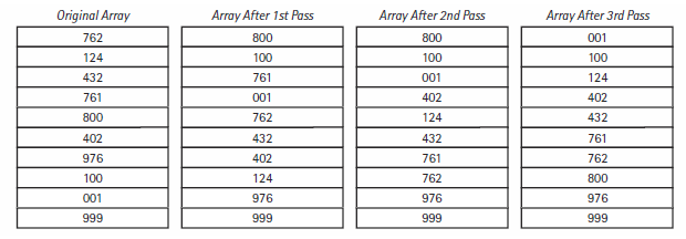
radix sort의 경우 array의 모든 원소가 숫자일 경우에 사용할 수 있는 정렬 방법으로 원소들끼리 비교하는 것이 아니라 원소의 자릿수끼리 비교하여 정렬하는 방식이다.
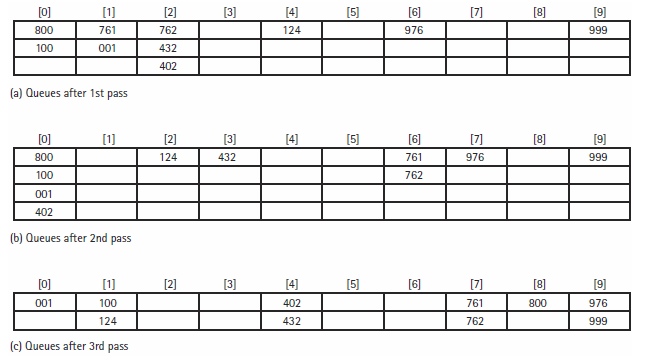
먼저 숫자가 특정 자리에 가질 수 있는 값은 0부터 9까지 10개이기 때문에 10개의 묶음을 구분하기 위한 queue를 10개의 index마다 생성한다.
그 후 배열의 모든 원소들을 탐색하면서 1의 자릿수가 n인 숫자는 n번째 index에 해당하는 queue에 저장하여 모든 원소들을 전부 저장한다.
그리고 0번째 index부터 순서대로 dequeue를 해서 1의 자리수가 오름차순으로 정렬된 array를 만든다.
이러한 과정을 요소 중에서 가장 길이가 긴 숫자의 자릿수만큼 반복하면 오름차순으로 정렬된 배열을 얻을 수 있다.
radix sort의 시간 복잡도를 계산해 보면 매 자릿수마다 $N$개의 요소들을 전부 탐색하고 이러한 과정을 요소들 중에서 자릿수가 가장 긴 요소의 자릿수인 $P$만큼 반복한다고 하면 총 $O(NP)$의 시간 복잡도가 걸린다.
따라서 만약 $P$ 가 매우 클 경우는 비효율적일 수 있지만 상황에 따라서는 가장 빠른 정렬 방법이 될 수도 있다.
- Stability
stability는 sorting 할 때 만약 array에 동일한 값이 있으면 해당하는 값들의 순서가 sorting을 끝나고도 동일하게 유지되는지 여부를 뜻한다.
위에서 설명한 정렬의 대부분의 경우 stability를 만족하지만 원소의 순서를 마음대로 바꾸는 heap sort와 quick sort의 경우 stability를 만족하지 않는다.
따라서 정렬의 조건으로 stability를 만족해야 하는 경우 위의 두 정렬 방법은 지양해야 한다.
'컴퓨터 > 자료구조' 카테고리의 다른 글
| 자료구조 - Searching (0) | 2023.12.02 |
|---|---|
| 자료구조 - DFS & BFS (Graph Searching) (1) | 2023.11.30 |
| 자료구조 - 그래프 (1) | 2023.11.30 |
| 자료구조 - 우선순위 큐(Priority Queue) (0) | 2023.11.29 |
| 자료구조 - Heap (1) | 2023.11.29 |


